Inverted File Product Quantization (IVF_PQ): Accelerate vector search by creating indices

Vector similarity search is finding similar vectors from a list of given vectors in a particular embedding space. It plays a vital role in various fields and applications because it efficiently retrieves relevant information from large datasets.

Vector similarity search requires excessive memory resources for efficient search, especially when dealing with dense vector datasets. Here comes the role of compressing High Dimensional vectors for optimizing memory storage. In this blog, We’ll discuss about

1. Product Quantization(PQ) & How it works
2. Inverted File Product Quantization(IVFPQ) Index
3. Implementation of IVFPQ using LanceDB

We’ll also see the performance of PQ and IVFPQ in terms of memory and cover an implementation of the IVFPQ Index using LanceDB.

Quantization is a process used for dimensional reduction without losing important information.

Quantization: Dimensionality Reduction

How does Product Quantization work?

Product Quantization can be broken down into steps listed below:

1. Divide a large, high-dimensional vector into equally sized chunks, creating subvectors.
2. Identify the nearest centroid for each subvector, referring to it as reproduction or reconstruction values.
3. Replace these reproduction values with unique IDs that represent the corresponding centroids.

Product Quantization

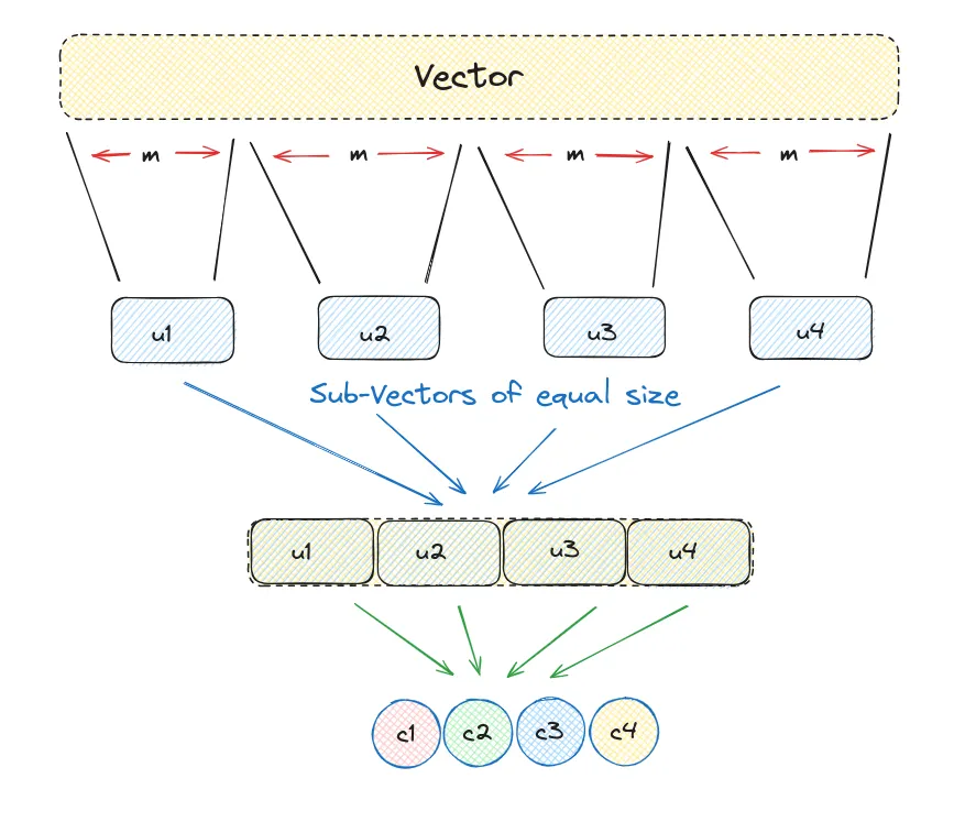
Let's see how it works in the implementation, of that we’ll create a random array of size 12 and keep the chunk size as 3.

import random

#consider this as a high dimensional vector
vec = v = [random.randint(1,20)) for i in range(12)]

chunk_count = 4
vector_size = len(vec)

# vector_size must be divisable by chunk_size
assert vector_size % chunk_count == 0
# length of each subvector will be vector_size/ chunk_count
subvector_size = int(vector_size / chunk_count)

# subvectors
sub_vectors = [vec[row: row+subvector_size] for row in range(0, vector_size, subvector_size)]
sub_vectors

The output looks like this

[[13, 3, 2], [5, 13, 5], [17, 8, 5], [3, 12, 9]]

These subvectors are substituted with a designated centroid vector called Reproduction Value because it helps identify each subvector. Subsequently, this centroid vector can be substituted with a distinct ID that is unique to it.

k = 2**5
assert k % chunk_count == 0
k_ = int(k/chunk_count)

from random import randint
# reproduction values
c = []  
for j in range(chunk_count):
    # each j represents a subvector position
    c_j = []
    for i in range(k_):
        # each i represents a cluster/reproduction value position 
       c_ji = [randint(0, 9) for _ in range(subvector_size)]
       c_j.append(c_ji)  # add cluster centroid to subspace list
    
  # add subspace list of centroids
    c.append(c_j)

#helper function to calculate euclidean distance
def euclidean(v, u):
    distance = sum((x - y) ** 2 for x, y in zip(v, u)) ** .5
    return distance

#helper function to create unique ids
def nearest(c_j, chunk_j):
    distance = 9e9
    for i in range(k_):
        new_dist = euclidean(c_j[i], chunk_j)
        if new_dist < distance:
            nearest_idx = i
            distance = new_dist
    return nearest_idx

Now, Let's see How we can get unique centroid IDs using the nearest helper function

ids = []
# unique centroid IDs for each subvector
for j in range(chunk_count):
    i = nearest(c[j], sub_vectors[j])
    ids.append(i)
print(ids)

Output shows unique centroid IDs for each subvector

[5, 6, 7, 7]

When utilizing PQ to handle a vector, we divide it into subvectors. These subvectors are then processed and linked to their closest centroids, also known as reproduction values, within the respective subclusters.

Instead of saving our Quantized Vector using the centroids, we substitute it with a unique Centroid ID. Each centroid has its specific ID, allowing us to later map these ID values back to the complete centroids.

quantized = []
for j in range(chunk_count):
    c_ji = c[j][ids[j]]
    quantized.extend(c_ji)

print(quantized)

Here is the reconstructed vector using Centroid IDs

[9, 9, 2, 5, 7, 6, 8, 3, 5, 2, 9, 4]

In doing so, we’ve condensed a 12-dimensional vector into a 4-dimensional vector represented by IDs. We opted for a smaller dimensionality for simplicity, which might make the advantages of this technique less immediately apparent.

It’s important to highlight that the reconstructed vector is not identical to the original vector. This discrepancy arises due to inherent losses during the compression and reconstruction process in all compression algorithms.

Let’s change our starting 12-dimensional vector made of 8-bit integers to a more practical 128-dimensional vector of 32-bit floats. By compressing it to an 8-bit integer vector with only eight dimensions, we strike a good balance in performance.

Original: 128×32 = 4096 Quantized: 8×8 = 64

This marks a substantial difference — a 64x reduction in memory.

How IVFPQ Index help in speeding things up?

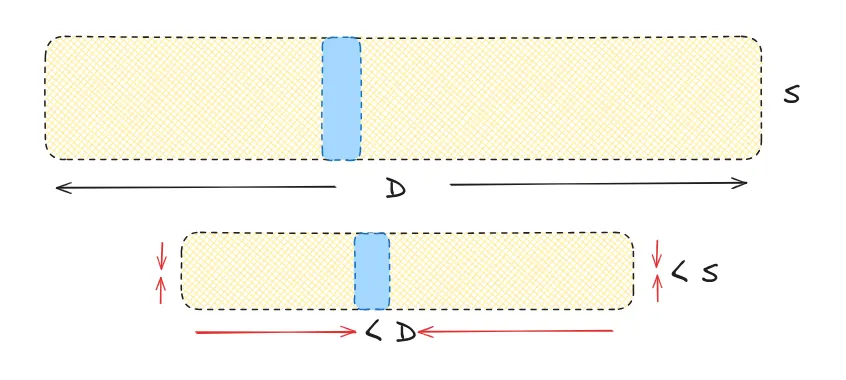
In IVFPQ, an Inverted File index (IVF) is integrated with Product Quantization (PQ) to facilitate a rapid and effective approximate nearest neighbor search by initial broad-stroke that narrows down the scope of vectors in our search.

After this, we continue our PQ search as we did before — but with a significantly reduced number of vectors. By minimizing our Search Scope, it is anticipated to achieve significantly improved search speeds.

IVFPQ can be very easily implemented in just a few lines of code using LanceDB

Creating an IVF_PQ Index

import lancedb
import numpy as np
uri = "./lancedb"
db = lancedb.connect(uri)

# Create 10,000 sample vectors
data = [{"vector": row, "item": f"item {i}"}
   for i, row in enumerate(np.random.random((10_000, 1536)).astype('float32'))]

# Add the vectors to a table
tbl = db.create_table("my_vectors", data=data)

# Create and train the index - you need to have enough data in the table for an effective training step
tbl.create_index(num_partitions=256, num_sub_vectors=96)

• metric (default: “L2”): The distance metric to use. By default, it uses Euclidean distance “L2". We also support "cosine" and "dot" distance as well.
• num_partitions (default: 256): The number of partitions of the index.
• num_sub_vectors (default: 96): The number of sub-vectors (M) that will be created during Product Quantization (PQ).

Now let's see what this IVF Index does to reduce the scope of vectors, Inverted file is an index structure that is used to map database vectors to their respective partitions where these vectors reside.

PQ vectors

Vectors are assigned to different Voronoi cells via IVF

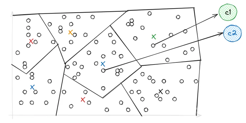
This is Voronoi's Representation of vectors using IVF, they’re simply a set of partitions each containing vectors close to each other, and when it comes to search — When we introduce our query vector, it restricts our search to the nearest cells only because of which searching becomes way faster compared to PQ.

Query Vector searches Closest cell

Afterwards, PQ needs to be applied as we have seen above.

All of this can be applied using the IVF+PQ Index using LanceDB in minimal lines of code

tbl.search(np.random.random((1536))) \
    .limit(2) \
    .nprobes(20) \
    .refine_factor(10) \
    .to_pandas()

• limit (default: 10): The number of results that will be returned
• nprobes (default: 20): The quantity of probes (sections) determines the distribution of vector space. While a higher number enhances search accuracy, it also results in slower performance. Typically, setting the number of probes (nprobes) to cover 5–10% of the dataset proves effective in achieving high recall with minimal latency.
• refine_factor (default: None): Refine the results by reading extra elements and re-ranking them in memory.
  A higher number makes the search more accurate but also slower.

Conclusion

It can be concluded that Product Quantization reduces memory consumption for storing high dimensional vectors and in addition to the IVF index, it extensively speeds up the process by searching in only the closest vectors.

Visit the LanceDB repo to learn more about lanceDB Python and Typescript library

To discover more such applied GenAI and vectorDB applications, examples and tutorials visit VectorDB-Recipes